#!pip install squarenet

import numpy as np
import matplotlib.pyplot as plt

from squarenet import SquareNet
from squarenet.sampler import samplepoints
from squarenet.utils import show_search_result

save_path = "sqrnet/plot" #for the plots

❒ SquareNet

Fitting our first dataset -1 million points randomly sampled on the 2D map of France

I = 1_000
N = I*I
points = samplepoints("france", size = (N, 2))
sn = SquareNet(gridshape = (I, I))
sn.fit(points, method = "robust")

Starting gridification... available method [fast, robust, ultimate]
selected robust

=== Carthesian sort ===
(max iter: 2 x 1000)
[█████████████████████████████] 1000/1000
[█████████████████████████████] 1000/1000


=== Final Status ===
succesfully sorted at iteration 220

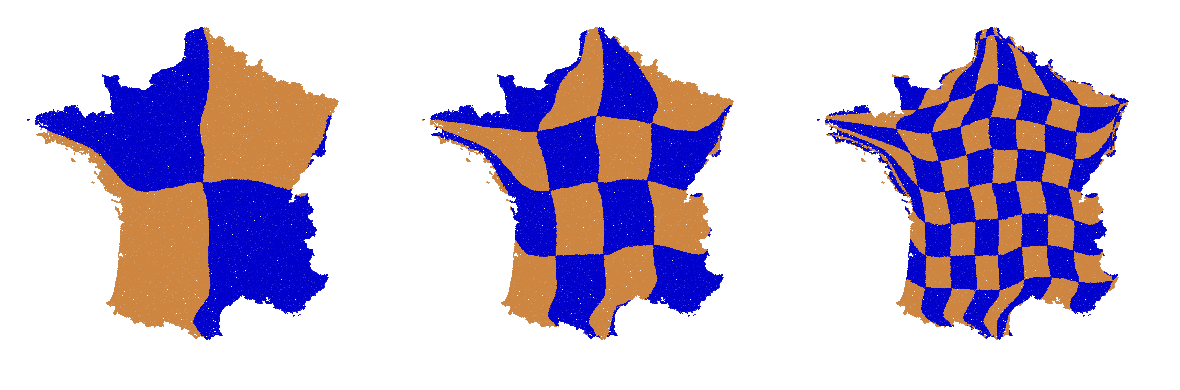
Now France is grided

sn.plot(style = "checkerboard", save_path = save_path) #should look like a checkerboard pattern

figure will be saved at sqrnet\plot.png

(<Figure size 1200x400 with 3 Axes>, None)

📡 Search Sorted:

Squarenet allow for a powerfull D-dimensional version of the 1D search sorted

#(x, y) coordinates of a random point in France
true_index = np.random.choice(N)
grid_multi_index = sn.mapidx(true_index)
point = points[true_index]

x, y = point[0], point[1]
print(f"random point x,y = ({x:.2f}, {y:.2f})\n\n")

#search sorted is a heuristic method that will find an
# (almost optimal) position in the grid that best
# fit the spatial coordinates of an unseen point.
# Augment n_iter to get better accuracy

#/!\ search sorted is fast, but will not give the exact nearest neighbor.

left_multi_index = sn.search_sorted(point, n_iter = 4, side = "left")
right_multi_index = sn.search_sorted(point, n_iter = 4, side = "right")

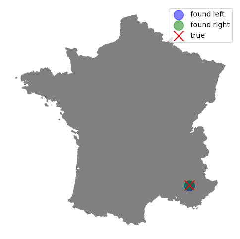
show_search_result(left_multi_index, right_multi_index, true_index, points, sn)

random point x,y = (0.83, 0.19)


true index (np.int32(863), np.int32(125))
with search sorted: [862 125] [864 126]

Fitting some holy dataset, again 1 million points in 2D

I = 1_000
N = I*I
points = samplepoints("holy", size = (N, 2))
sn = SquareNet(gridshape = (I, I))

sn.fit(points)

Starting gridification... available method [fast, robust, ultimate]
selected fast

=== Carthesian sort ===
(max iter: 1000)
[█████████████████████████████] 1000/1000

=== Final Status ===
succesfully sorted at iteration 16

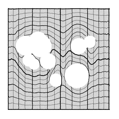
sn.plot(style = "mesh", save_path = save_path)

figure will be saved at sqrnet\plot_1.png

(<Figure size 400x400 with 1 Axes>, None)

⚛️ Neighbormap

Neighbormap provides a fast diagnostic of grid quality by estimating how close

true nearest neighbors remain in grid-index space.

In the printed neighbormap, in each cell you will find how many points Y were the nearest neighbor

of the central points X in that particular cell relative to X cell, accros 20 million evenly sampled pairs (X, Y).

If you need the matrix to compute something on it (instead of just a print) or to give a custom distance kernel etc:

from squarenet.neighbormap import neighbormap

-> more parameters and more control

sn.neighbormap(log2 = False)

neighbor map on axes (0, 1)
                                                               1
                                                                         1              1
   1                   1         1                   1              1              2         1                        1         1
                  1    1    1         1    3    4    5    3   11   15   18    9   14   13    3    2         1    2    1         2    1         1    1
                       1    1    1    1    3   11   18   34   88  172  315  381  293  166   71   21   15   11    2    3    2    3    4         1
                                           3    5   27   73  276  846 2464 4262 2444  790  206   56   20   13    8    2         1
                                                          7   95 1090 6434    ■ 6265 1124   83    6
                  1              2    2    7    9   28   53  216  822 2391 4280 2535  868  250   68   23    5    1
             2         1    1    1    4    4   11   23   28   58  156  311  346  327  175   60   32   14   11    5    2
             3    3    1         1    2    3    2    1    3    6   11   21   11   15   19    8    5    3    6              1                   1    1
                       1         1    1                             1              4    1         1    1    2                        1
        1                                       1                                                      1    1

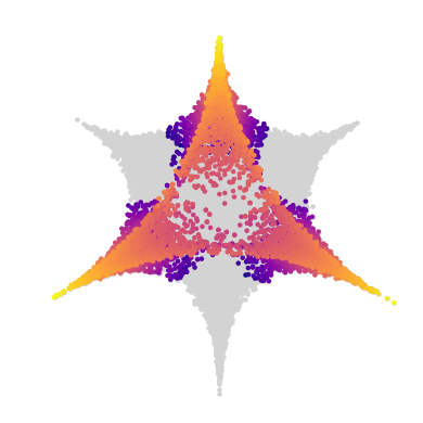
Fitting something spiky (1million points, 3D).

I = 100
N = I*I*I
points = samplepoints("spiky", size = (N, 3))
sn = SquareNet(gridshape = (I, I, I))

sn.fit(points, method = "robust")

Starting gridification... available method [fast, robust]
selected robust

=== Carthesian sort ===
[█████████████████████████████] 100/100

=== Final Status ===
succesfully sorted at iteration 120

sn.plot(animate = True, style = "scatter", save_path = save_path)

figure will be saved at sqrnet\plot.gif
ffmpeg unavailable. Npoints = 1000000 and style is 'scatter' -> could take 1/2 minutes

(<Figure size 400x400 with 1 Axes>,
 <matplotlib.animation.FuncAnimation at 0x1e7007a3050>)

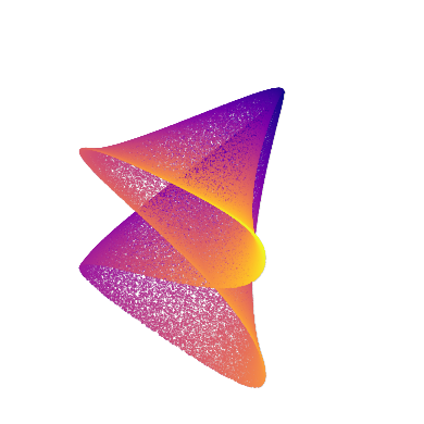
Fitting a Manifold (1million points, 2d latent loop in a 4D space). Just put 1 for some of the grid dimensions

I = 1_000
N = I*I*1*1
points = samplepoints("4Dloop", size = (N, 4))
sn = SquareNet(gridshape = (I, I, 1, 1))

sn.fit(points)

Starting gridification... available method [fast, robust]
selected fast

=== Carthesian sort ===
[█████████████████████████████] 100/100

=== Final Status ===
succesfully sorted at iteration 30

sn.plot(style = "scatter", animate = True, save_path = save_path)

figure will be saved at sqrnet\plot_1.gif
ffmpeg unavailable. Npoints = 1000000 and style is 'scatter' -> could take 1/2 minutes

(<Figure size 400x400 with 1 Axes>,
 <matplotlib.animation.FuncAnimation at 0x1e7007a3c50>)

⏱ Practical trade-off

Exploring with fast, robust and ultimate method, you will find following empiricall caracteristics:

Method	Quality (NN locality)	Speed	Stability	Recommended use
fast	medium	very high	axis-biased	large-scale / preprocessing
robust	high	high	balanced	default choice
ultimate*	very high	low	most stable	offline high-quality grids

⚠️ Ultimate method needs a suffisant (potentially very high) max iter parameter to give the best results.

Max_iter is default to 1000 which is good in many cases for small/medium number of points, but for datasets

with more than 1 Million points and a tricky geometry 10_000 iterations will be neaded to be safely

considered as optimal, wich would lead to a 20 minutes long fit.

➡️ 02. JAX and PyTorch